Common Image Processing Tools
Image Thresholding
The simplest method of segmenting a gray-scale image
is to threshold it. By selecting a certain value, and
setting all pixel values below it to one (white), and
all pixel values above it to zero (black), we get
a binary image. From the histogram we see
that the pixel values of the characters are usually below 80.
We'll first try to threshold the image with a low value
to minimize the background noise: [figure X5] is thresholded
with value 65. The writing is unreadable.
Using a larger value, 80, suggested by the histogram [figure X4],
we have [figure X6]. The writing is quite readable,
with some of the background still left. Parts of the
last character are missing, so we'll try yet another
threshold value, 100, and end up with [figure X7]. Here,
the last character is easier to identify, but the first
characters are beginning to disappeaar into the background.
If the background could be separated from the writing
with a certain grey scale value, image thresholding would
be the only method needed for processing the images.
Of all our digitized images, none of them could perfectly
be segmented using thresholding; there were always
parts of characters missing, or background blurred
the characters. But for a properly chosen threshold value,
the writing was quite readable.
The best threshold value changes from an image to another.
It is also dependent of location, because some parts of the
text are darker or lighter than others. So, the larger the
image, the harder it is to choose a globally acceptable
threshold value. A good estimate can easily be found by
examining histograms (or single pixel values) of areas
inside characters and choosing an upper boundary appropriately.
The best value can be quickly found manually,
because the process is very quick. Because the writing
does not show up in a global histogram, it is hard to
find a way for automatic selection of a good threshold value.
One could estimate a ratio between the number of character
pixels and background pixels in an average image, and
use it to select a cutoff point, for the first approximation.
Figure 32:
Sample image, thresholded at 65.
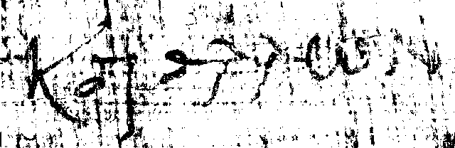 Figure 33:
Sample image, thresholded at 80.
Figure 33:
Sample image, thresholded at 80.
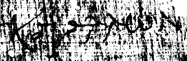
Figure 34:
Sample image, thresholded at 100.
Histogram Modification
One of the best ways to improve contrast without loosing
much information and too many grey levels is to use histogram-
modification. This technique re-maps the original grey levels
to anothers according to a mapping function.
One can re-map the grey levels very quickly by a
statistically optimal algorithm (equalization) or
manually. Many image processing programs,
like Adobe Photoshop ©, have very easy to use tools
available for this. If the mapping function is
monotonically increasing, the order of pixel values
is preserved, and the process is purely contrast-modifying.
The automatic histogram equalization
method stretches the grey levels of a given image
so that it is as equally possible for any given pixel
to be of any gray scale value; i.e. the number of pixels belonging
to any grey level is equal.
The histogram mapping function is typically presented as a
curve, original greyscale values on x-axis and their mapped
values on y-axis. The grey levels at the area of interest,
in this case the grey levels of characters, can be
dynamically separated from other areas by applying a steep
mapping curve to that area.
The method is very good in enhancing contrast. Figures [X8] show
the test figure [X5] optimally equalized [X8a],
and the new, stretched histogram [X8b].
A manually adjusted version can be seen in [figure X10a]
with resulting histogram [X10c].
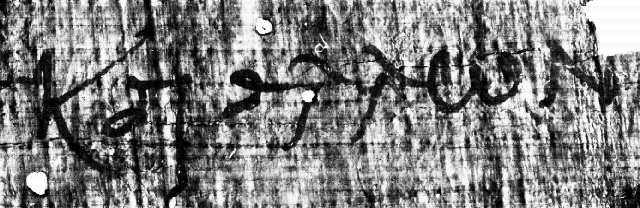
Figure 35a:
Sample image, histogram equalized.
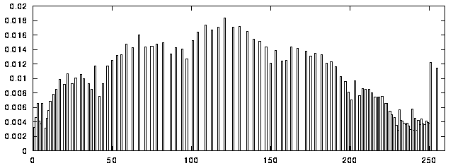 Figure 35b:
Histogram of sample image after equalization (compare to pic. X3).
Figure 35b:
Histogram of sample image after equalization (compare to pic. X3).
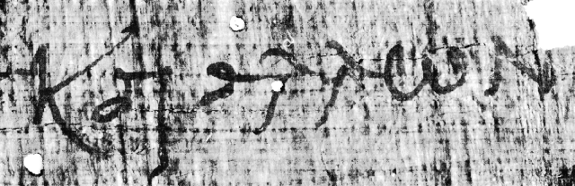
Figure 36a:
Sample image, manually equalized.
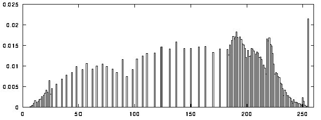 Figure 36b:
Histogram of sample image after manual histogram modification.
Figure 36b:
Histogram of sample image after manual histogram modification.
Edge Detection
Edge detection algorithms search for rapid changes
of pixel values. These operators are typically
different kinds of first or second order derivatives.
Results of several differential operators can bee seen in
figures [37] (horizontal derivative), [38] (vertical derivative),
[39] (sum of horizontal and vertical derivatives) and
[40] (the square environment derivative).
These images are histogram-equalized, because resulting
values of these operators are typically very low,
and the images therefore very dark. The edges
of the characters are visible, but unluckily
the background noise is too. The cyclic error
of the scanner's 4th bit that causes peaks every
16 grey levels might show up when applying these algorithms.
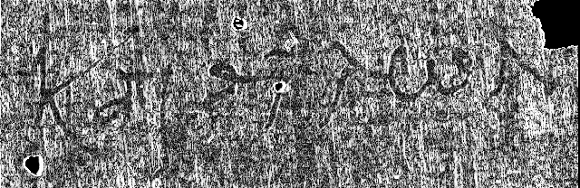
Figure 37:
Horizontal derivative of the sample image (histogram equalized).
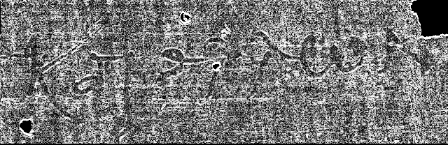 Figure 38:
Vertical derivative of the sample image (histogram equalized).
Figure 38:
Vertical derivative of the sample image (histogram equalized).
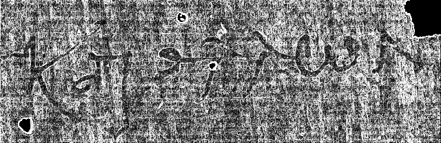
Figure 39:
Sum of X-and Y-derivatives of the sample image (histogram equalized).
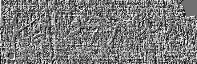 Figure 40:
Square-environment derivative of the sample image (histogram equalized).
Figure 40:
Square-environment derivative of the sample image (histogram equalized).
Noise Reduction
Noise in a grayscale image is usually understood
as single pixels or very small areas containing very different
grayscale values from their environment. Averaging
is probably the most basic noise reduction method.
One can choose, say, a 5x5 pixel matrix, calculate the
average of all the 25 pixels, and set the value of
the middle pixel to that [figure X].
The averaged image is blurry, and, especially,
sharp edges are lost.
One can modify the algorithm by setting a threshold to
it, so that the value of the middle pixel is changed
only when its value is very different from the average,
or use the average with weighting factor. The shape of the matrix
can also be varied from square to, say, hexagonal, or a cross.
A better way to reduce noise is by using order-based
statistical filters such as the median filter.
These filters, or algorithms, arrange the grayscale values
of a chosen area in increasing order, and set one of
these values to the current pixel value. Basic median filter
chooses the middle value. These filters can be biased
to select some other value or the pixels involved can be
weighted. Figure [X] shows the test image median-filtered
with a 5x5 matrix.
Figure 41:
Sample image, averaged with 5x5 matrix.
 Figure 42:
Sample image, median filtered with 5x5 matrix.
Figure 42:
Sample image, median filtered with 5x5 matrix.
Deviation Method
Suppose that the writing on a papyrus covers the structural
features of the carbonized papyrus surface, and that the writing
is nearly equally colored with less disturbances than the
background. In that case, we could distinguish the writing
with a filter that detects the deviation or variance of a
chosen area. The deviation inside a character shuld be small,
and large outside. Also, the edges of the characters would
be enhanced, because there the deviation would be quite large.
[Figure X] shows the deviation of the
sample image using an 7x7 matrix. The edges are enhanced,
but the deviation inside and outside the characters seems
to be equally small, so that it cannot really be used
to distinguish the writing from the background. The
enhancement of the edges, howewer, is good. The variance
(7x7 pixels) is shown in [figure 43].
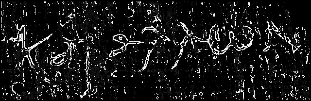
Figure 43:
Deviation of sample image
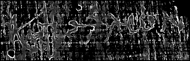 Figure 44:
Variance of sample image
Figure 44:
Variance of sample image
Papyrus Structure Elimination
The papyrus sheet is made from horizontal and vertical papyrus
stripes. These stripes, and the cell structure, can be seen
in any piece of papyrus, and also in our carbonized fragments.
Vertical and horizontal lines can be detected, for example,
by comparing a line to the average of its left-and right-hand
square environments and searching for a large difference.
If the width of these lines vary much, simple line detectors
are not so efficient. We tried to reduce the vertical structure
by calculating the averages of pixel values of each vertical line,
and then subtracting these averages from the original image.
Many of the disturbing lines were removed, and the original
figure wasn't otherwise altered too much [figure X]
(the slope of vertical lines was estimated and accounted for).
The removal of the structure is indeed very discreet;
all small details remain, and it may even be difficult
to spot the differences to the original picture. As a test,
we asked several people to spot the differences between
the original and the image from which vertical structure was
eliminated; none of them found the differences. This means,
on the one hand, that the removal didn't alter too much the
pictures, but on the other, that the readability was not so
much improved. Most of the visible background structure is local,
so that the removal of averaged lines really removes only
the longest and straightest ones.
The papyrus background structure is not always purely vertical
and horizontal. In our sample picture, for example, the vertical
lines are tilted about 6 ° (one pixel to the right every
10 pixels). A simple algorithm for detecting
the direction of axes could compare successive lines,
testing them by shifting the previous line horizontally
by -1, 0, or 1 pixels, and choosing the shift as the
one wich causes least difference to the current line
(in least square error sense, for example).
The average slope would be the average of all the shifts.
Some rules should be applied to the process to prevent it
from too strong deviations. One could apply momentum, for
example, to keep the changes of the shifts small.
There is also other ways to find the major axes of a
picture, like correlation.
The problems with this kind of structure elimination are
related to the way the averages are calculated, and
to the structure itself. If characters or large parts of
them are tilted along the structural lines, they may affect
the calculation of the average and be also reduced from the
pictures. Also, some of the structural lines are not continuous,
and can be short compared to the size of the characters,
so that they cannot effectively be reduced using this algorithm.
Figure 45:
The original sample image.
 Figure 46:
Sample image, vertical structure eliminated.
Figure 46:
Sample image, vertical structure eliminated.

Figure 47:
Sample image, horizontal structure eliminated.
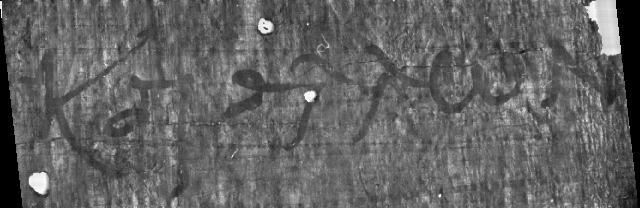 Figure 48:
Sample image, horizontal and vertical structures eliminated (in
this order).
Figure 48:
Sample image, horizontal and vertical structures eliminated (in
this order).
FFT Filters
Fourier transformation allows us to handle the pictures
in frequency domain insteadt of spatial domain. The simplest
Fourier filters are low-pass and high-pass filters,
which filter out high or low frequencies (rapid changes
in pixel values or average values). A notch filter
cancels only certain frequencies. The effect of a low-
pass filter is blurring, noise-reducting. The high-pass
filter cancels the overall grey values, emphasizing edges
and noise. Proper filters in frequency domain could reduce
the vertical and horizontal lines and enhance edges of
characters. The drawback of filters using Fourier
transformations is the need for very complex and slow
calculations. Further experiments are encouraged.
Miscellaneous Viewing
There are many different simple viewing tools along with these
filters. Many new views to the images can be found by
histogram (or color map) manipulation. The grey level map
can be reversed to turn the pictures to their negatives,
it can be rotated, pseudo-coloured, or multiplied. Every
method may give some new information, so that one should
not count any of them out.
 Back to Image Processing
 Back to Contents
 Next: Filter Combinations
Antti Nurminen, 34044T, andy@cs.hut.fi
laplacian (F(x,y)=dx ²+dy²), [figure X] - sobel.